Soham Bhattacharyya MASc, ECE Notes, pointers and cheatsheets.

How I made pdf2wav

By constructing a pipeline of pdf reader stream to FastPitch spectrogram generator to MelGAN vocoder. pdf2wav can convert any pdf(, doc, txt, etc.) file to wav(, flac, mp3, etc.) audio file. This can be used as an audiobook generator.

Samples:

/assets/audio/pdf2wav.wav

Wordle of the Day!

[SPOILER ALERT] https://multivac64.pythonanywhere.com/

Wordle of the Day! feature image Photo Credit: powerlanguage.co.uk/wordle

A Visualization of Riemann Zeta Function

This is a visualization of how the Riemann zeta function transforms the complex s-plane. We assume analytic continuation. Precision is 53 significant decimal digits.

  • Samples from complex s-plane:

https://web.cs.dal.ca/~soham/viz-s.html

  • Transformed s-plane:

https://web.cs.dal.ca/~soham/viz-zeta.html

A Visualization of Riemann Zeta Function feature image

Runtime Computation Times - Functions versus Operator

A test on integer and float exponentials can be run to get the computation times.

print(timeit.timeit(stmt="pow(2, 100)"))
1.30916247735
print(timeit.timeit(stmt="pow(2, 1023)"))
3.69032251306
print(timeit.timeit(stmt="math.pow(2, 100)", setup='import math'))
0.322029196449
print(timeit.timeit(stmt="math.pow(2, 1023)", setup='import math'))
0.334137509097
print(timeit.timeit(stmt="pow(2.01, 1016)"))
0.302062482802
print(timeit.timeit(stmt="math.pow(2.0, 1023)", setup='import math'))
0.310684528341
print(timeit.timeit(stmt="math.pow(2.01, 1016)", setup='import math'))
0.310034306037

Now, see the fall while using the operator.

print(timeit.timeit(stmt="2 ** 1023"))
0.0310322261626
print(timeit.timeit(stmt="2.0 ** 1023"))
0.0324852041249
print(timeit.timeit(stmt="2.01 ** 1016"))
0.0302783594007
print(timeit.timeit(stmt="2.01 ** 1016.01"))
0.0301967149462

This apparent time difference at runtime occurs most likely due to the overhead function call procedure. Disassembling to bytecodes gives an insight.

dis.dis('2.01 ** 1016')
  1           0 LOAD_CONST               2 (1.1147932725682862e+308)
              2 RETURN_VALUE
dis.dis('pow(2.01, 1016)')
  1           0 LOAD_NAME                0 (pow)
              2 LOAD_CONST               0 (2.01)
              4 LOAD_CONST               1 (1016)
              6 CALL_FUNCTION            2
              8 RETURN_VALUE
dis.dis('math.pow(2.01, 1016)')
  1           0 LOAD_NAME                0 (math)
              2 LOAD_ATTR                1 (pow)
              4 LOAD_CONST               0 (2.01)
              6 LOAD_CONST               1 (1016)
              8 CALL_FUNCTION            2
             10 RETURN_VALUE

Also, as a food for thought, notice that while the performance of the inbuilt pow function depends upon the numerics given in the arguments, the math.pow acts mostly indifferent.

A Bunch of Cheatsheets

I will try to keep this post updated.

A Bunch of Cheatsheets feature image Photo Credit: Eric Rowell

Some Key-Points on \(z\)-Transform, Frequency-Domain and Digital Filters

[Under Build]

I have tried to jot down some of the most used concepts in as compact form as possible.

Introduction to DSP using MATLAB - Part IV - References

[Under Build]

Introduction to DSP using MATLAB - Part III

A link to the previous part, a link to the first part and a link to the references part.

25-tap Lowpass Filter using Rectangular and Hamming Windows

The rectwin and hamming functions create the rectangular and Hamming window.

Rectangular window from wikimedia Hamming window from wikimedia

The Hamming window is generated from the equation: \[w(n) = 0.54 - 0.46 cos\left(2\pi\frac{n}{N}\right), \qquad 0 \le n \le N\] The window length \(L = N + 1\).

%% To design a 25-tap lowpass filter with cutoff frequency .5pi radians
% using rectangular and Hamming windows and plot their frequency response
wc = .5*pi;      % Cutoff frequency
N = 25; alpha = (N-1)/2; eps = .001;
n = 0:1:N-1;
hd = sin(wc*(n-alpha+eps))./(pi*(n-alpha+eps));
wr = rectwin(N); % Rectangular window sequence
hn = hd.*wr';    % Filter coefficients
w = 0:.01:pi;
h = freqz(hn,1,w);
plot(w/pi,abs(h)); hold on
wh = hamming(N); % Hamming window sequence
hn = hd.*wh';    % Filter coefficients
w = 0:.01:pi;
h = freqz(hn,1,w);
plot(w/pi,abs(h),'-.'); grid;
xlabel('Normalized frequency \omega/\pi');
ylabel('Magnitude'); hold off

Frequency response of 25-tap lowpass filter using rectangular and Hamming windows

25-tap Highpass Filter using Rectangular and Blackman Windows

The blackman function creates the Blackman window.

Blackman window from wikimedia

The following equation defines the Blackman window of length \(N\): \[w(n) = 0.42 - 0.5 cos\frac{2\pi n}{N - 1} + 0.08cos\frac{4\pi n}{N - 1}, \] \[0 \le n \le M - 1\] where \(M\) is \(N/2\) for \(N\) even and \((N + 1)/2\) for \(N\) odd.

%% To design a 25-tap highpass filter with cutoff frequency .5pi radians
% using rectangular and Blackman windows and plot their frequency response
wc = .5*pi;      % Cutoff frequency
N = 25; alpha = (N-1)/2; eps = .001;
n = 0:1:N-1;
hd = (sin(pi*(n-alpha+eps)) - sin(wc*(n-alpha+eps))) ./ (pi*(n-alpha+eps));
wr = rectwin(N); % Rectangular window sequence
hn = hd.*wr';    % Filter coefficients
w = 0:.01:pi;
h = freqz(hn,1,w);
plot(w/pi,abs(h)); hold on
wh = blackman(N); % Blackman window sequence
hn = hd.*wh';     % Filter coefficients
w = 0:.01:pi;
h = freqz(hn,1,w);
plot(w/pi,abs(h),'-.'); grid;
xlabel('Normalized frequency \omega/\pi');
ylabel('Magnitude'); hold off

Frequency response of 25-tap highpass filter using rectangular and Blackman windows

25-tap Bandpass Filter using Rectangular and Hamming Windows

%% To design a 25-tap bandpass filter with cutoff frequency .25pi and .75pi radians
% using rectangular and Hamming windows and plot their frequency response
wc1 = .25*pi; wc2 = .75*pi;      % Cutoff frequency
N = 25; a = (N-1)/2;
eps = .001; % To avoid indeterminate form
n = 0:1:N-1;
hd = (sin(wc2*(n-a+eps)) - sin(wc1*(n-a+eps))) ./ (pi*(n-a+eps));
wr = rectwin(N); % Rectangular window sequence
hn = hd.*wr';    % Filter coefficients
w = 0:.01:pi;
h = freqz(hn,1,w);
plot(w/pi,abs(h)); hold on
wh = hamming(N); % Hamming window sequence
hn = hd.*wh'; % Filter coefficients
w = 0:.01:pi;
h = freqz(hn,1,w);
plot(w/pi,abs(h),'-.'); grid;
xlabel('Normalized frequency \omega/\pi');
ylabel('Magnitude'); hold off

Frequency response of 25-tap bandpass filter using rectangular and Hamming windows

25-tap Bandstop Filter using Rectangular and Hamming Windows

%% To design a 25-tap bandstop filter with cutoff frequency .25pi and .75pi radians
% using rectangular and Hamming windows and plot their frequency response
wc1 = .25*pi; wc2 = .75*pi;      % Cutoff frequency
N = 25; a = (N-1)/2;
eps = .001; % To avoid indeterminate form
n = 0:1:N-1;
hd = (sin(wc1*(n-a+eps)) - sin(wc2*(n-a+eps)) + sin(pi*(n-a+eps))) ./ (pi*(n-a+eps));
wr = rectwin(N); % Rectangular window sequence
hn = hd.*wr';    % Filter coefficients
w = 0:.01:pi;
h = freqz(hn,1,w);
plot(w/pi,abs(h)); hold on
wh = hamming(N); % Hamming window sequence
hn = hd.*wh';    % Filter coefficients
w = 0:.01:pi;
h = freqz(hn,1,w);
plot(w/pi,abs(h),'-.'); grid;
xlabel('Normalized frequency \omega/\pi');
ylabel('Magnitude'); hold off

Frequency response of 25-tap bandstop filter using rectangular and Hamming windows

25-tap Hilbert Transformer using Bartlett and Hamming Windows

Triangular window from wikimedia

The coefficients of a Bartlett window are computed as follows: \[w(n) = \begin{cases} \frac{2n}{N}, & \text{\(0 \le n \le \frac{N}{2}\)} \\[2ex] 2-\frac{2n}{N}, & \text{\(\frac{N}{2} \le n \le N\)} \end{cases} \] The window length \(L = N + 1\).

%% To design a 25-tap Hilbert transformer using Bartlett
%  and Hamming windows and plot their frequency response
N = 25; a = (N-1)/2; eps = .001;
n = 0:1:N-1;
hd = (1 - cos(pi*(n-a+eps))) ./ (pi*(n-a+eps)); hd(a+1) = 0;
wt = bartlett(N); % Bartlett window
hn = hd.*wt';     % Filter coefficients
w = 0:.01:pi;
h = freqz(hn,1,w);
plot(w/pi,abs(h));   hold on
wh = hamming(N); % Hamming window sequence
hn = hd.*wh';    % Filter coefficients
w = 0:.01:pi;
h = freqz(hn,1,w);
plot(w/pi,abs(h),'-.'); grid;
xlabel('Normalized frequency \omega/\pi');
ylabel('Magnitude'); hold off

Frequency response of 25-tap Hilbert transformer using Bartlett and Hamming windows

25-tap Differentiator using Rectangular, Bartlett and Hann Windows

Hann window from wikimedia

The following equation generates the coefficients of a Hanning window: \[w(n) = 0.5\left(1−cos\left(2\pi\frac{n}{N}\right)\right), \qquad 0 \le n \le N\] The window length \(L = N + 1\).

%% To design a 25-tap differentiator using rectangular, Bartlett
%  and Hanning windows and plot their frequency response
N = 25; a = (N-1)/2; eps = .001;
n = 0:1:N-1;
hd = cos(pi*(n-a)) ./ (pi*(n-a)); hd(a+1) = 0;
wr = rectwin(N);  % rectangular window
hn = hd.*wr';     % Filter coefficients
w = 0:.01:pi;
h = freqz(hn,1,w);
plot(w/pi,abs(h),'-.'); hold on
wt = bartlett(N); % Bartlett window
hn = hd.*wt';     % Filter coefficients
w = 0:.01:pi;
h = freqz(hn,1,w);
plot(w/pi,abs(h),'--'); hold on
wh = hann(N); % Hanning window sequence
hn = hd.*wh'; % Filter coefficients
w = 0:.01:pi;
h = freqz(hn,1,w);
plot(w/pi,abs(h),'-');  grid;
xlabel('Normalized frequency \omega/\pi');
ylabel('Magnitude');    hold off

Frequency response of 25-tap differentiator using rectangular, Bartlett and Hanning windows

FIR Lowpass Filter using Hamming and Blackman Windows

The following equation defines the Blackman window of length N: \[w(n) = 0.42 − 0.5 cos\frac{2\pi n}{N - 1} + 0.08 cos\frac{4\pi n}{N - 1}, \] \[0 \le n \le M - 1\] where \(M\) is \(N/2 \) for \(N\) even and \((N + 1)/2 \) for \(N\) odd.

%% To design an FIR lowpass filter using Hamming and Blackman windows
wc = 0.5*pi; % Cutoff frequency
N = 25;
b = fir1(N,wc/pi,hamming(N+1));
w = 0:.01:pi;
h = freqz(b,1,w);
plot(w/pi,abs(h));   hold on
b = fir1(N,wc/pi,blackman(N+1));
w = 0:.01:pi;
h = freqz(b,1,w);
plot(w/pi,abs(h),'-.'); grid;
xlabel('Normalized frequency \omega/\pi');
ylabel('Magnitude'); hold off

FIR lowpass filter using Hamming and Blackman windows

Lowpass Filter using Kaiser Window

Kaiser window from wikimedia where \(\beta =^{def} \pi\alpha\). 
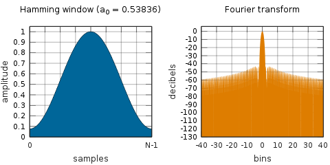
The coefficients of a Kaiser window are computed from the following equation: \[w(n) = \frac{I_0\left(\beta\sqrt{1 - \left(\frac{n - N/2}{N/2}\right)^2}\right)}{I_0(\beta)}, \qquad 0 \le n \le N\] where \(I_0\) is the zeroth-order modified Bessel function of the first kind. The length \(L = N + 1\).

%% To plot the frequency response of lowpass filter using Kaiser window
%  for different values of beta
wc = 0.5*pi; % Cutoff frequency
N = 25;
b = fir1(N,wc/pi,kaiser(N+1,.5));   %Beta = .5
w = 0:.01:pi;
h = freqz(b,1,w);
plot(w/pi,20*log10(abs(h)));      hold on
b = fir1(N,wc/pi,kaiser(N+1,3.5));  %Beta = 3.5
w = 0:.01:pi;
h = freqz(b,1,w);
plot(w/pi,20*log10(abs(h)),'-.'); hold on
b = fir1(N,wc/pi,kaiser(N+1,8.5));  %Beta = 8.5
w = 0:.01:pi;
h = freqz(b,1,w);
plot(w/pi,20*log10(abs(h)),'--'); grid;
xlabel('Normalized frequency \omega/\pi');
ylabel('Magnitude');              hold off

Frequency response of lowpass filter using Kaiser window

FIR Lowpass Filter using Frequency Sampling Method

%% To design a FIR lowpass filter with cutoff frequency .5pi using frequency sampling method
N = 33; % Number of samples
alpha = (N-1)/2;
Hrk = [ones(1,9), zeros(1,16), ones(1,8)]; % Samples of magnitude response
k1 = 0:(N-1)/2; k2 = (N+1)/2:N-1;
theta_k = [(-alpha*(2*pi)/N)*k1,(alpha*(2*pi)/N)*(N-k2)];
Hk = Hrk.*(exp(1i*theta_k));
hn = real(ifft(Hk,N));
w = 0:.01:pi;
H = freqz(hn,1,w);
plot(w/pi,20*log10(abs(H))); hold on
% FIR filter design using frequency sampling method with a transition sample
% at Hk(9) = 0.5 and Hk(24) = 0.5
Hrk = [ones(1,9), 0.5, zeros(1,14), 0.5, ones(1,8)]; % Samples of magnitude response
k1 = 0:(N-1)/2; k2 = (N+1)/2:N-1;
theta_k = [(-alpha*(2*pi)/N)*k1, (alpha*(2*pi)/N)*(N-k2)];
Hk = Hrk.*(exp(1i*theta_k));
hn = real(ifft(Hk,N));
w = 0:.01:pi;
H = freqz(hn,1,w);
plot(w/pi,20*log10(abs(H)),'-.'); grid;
xlabel('Normalized frequency \omega/\pi');
ylabel('Magnitude');         hold off

FIR lowpass filter using frequency sampling method

FIR Lowpass Filter using Kaiser Window

%% To design an FIR lowpass filter for the given specifications using Kaiser window
alphap = 0.1; % Passband attenuation in dB
alphas = 44;  % Stopband attenuation in dB
ws = 30;      % Stopband frequency in rad/sec
wp = 20;      % Passband frequency in rad/sec
wsf = 100;    % Sampling frequency in rad/sec
B = ws - wp;  % Transition width
wc = 0.5*(ws+wp);  % Cutoff frequency in rad/sec
wcr = wc*2*pi/wsf; % Cutoff drequenct=y in rad
D = (alphas - 7.95) / 14.36;
N = ceil((wsf*D/B)+1); % Order of the filter
alpha = (N-1) / 2
gamma = (.5842*(alphas-21).^(0.4)+0.07886*(alphas-21));
n = 0:1:N-1;
hd = sin(wcr*(n-alpha)) ./ (pi*(n-alpha)); hd(alpha+1) = 0.5;
wk = (kaiser(N,gamma))';
hn = hd.*wk;
w = 0:.01:pi;
h = freqz(hn,1,w);
subplot(2,1,1), plot(w/pi,20*log10(abs(h)))
xlabel('Normalized frequency \omega/\pi'); ylabel('Magnitude');
subplot(2,1,2), plot(w/pi,angle(h))
xlabel('Normalized frequency \omega/\pi'); ylabel('Magnitude');

FIR lowpass filter using Kaiser window

This repo contains all the scripts used in this post. Here is a link to the previous part, a link to the first part and a link to the references part.

Introduction to DSP using MATLAB - Part II

A link to the previous part, a link to the next part and a link to the references part.

DFT of a Sequence - Magnitude and Phase Response

The function takes the input sequence and the number of frequency points as two arguments.

%% DFT of a sequence and plot of the magnitude and phase response
x = ones(1,4); %Input sequence
N1 = 8; %Number of frequency points
Y1 = dft(x,N1)
k = 0:1:N1-1;
subplot(2,2,1), stem(k,abs(Y1)), xlabel('k'), ylabel('|Y1(k)|');
subplot(2,2,3), stem(k,angle(Y1)), xlabel('k'), ylabel('arg(Y1(k))');
N2 = 31 %Number of frequency points
Y2 = dft(x,N2)
k = 0:1:N2-1;
subplot(2,2,2), stem(k,abs(Y2)), xlabel('k'), ylabel('|Y2(k)|');
subplot(2,2,4), stem(k,angle(Y2)), xlabel('k'), ylabel('arg(Y2(k))');

dft.m:

function X = dft(xn,N)
% To compute the DFT of the sequence x(n)
L = length(xn); %Length of the sequence
%Checking for the length of the DFT
if(N<L)
    error('N must be >=L')
end
x1 = [xn zeros(1,N-L)]; %Appending zeros
%Computation of twiddle factors
for k = 0:1:N-1
    for n = 0:1:N-1
        p = exp(-i*2*pi*n*k/N);
        x2(k+1,n+1) = p;
    end
end
X = x1 * x2;

Notice that the Command Window shows the two output sequences of the 8-point and 50-point DFT.

Magnitude and phase response of the DFT of a sequence

Inverse DFT of a Sequence

%% Inverse DFT of a sequence
X = [4,1+i,0,1,-i,0,1+i,1-i];
N = length(X);
xn = idft(X,N)

idft.m:

function xn = idft(X,N)
%To compute the inverse DFT of the sequence X(k)
L = length(X); %Length of the sequence
%Computation of twiddle factors
for k = 0:1:N-1
    for n = 0:1:N-1
        p = exp(i*2*pi*n*k/N);
        x2(k+1,n+1) = p;
    end
end
xn = (X*x2.')/N;

Command Window output:

xn =
  Columns 1 through 7
   1.0000 + 0.0000i   0.5366 + 0.0884i   0.1250 - 0.3750i   0.1098 + 0.3384i   0.2500 + 0.0000i   0.7134 - 0.0884i   0.6250 - 0.1250i
  Column 8
   0.6402 + 0.1616i

Circular Convolution of two Sequences

%% Circular convolution of two sequences
n = 0:7;
x = sin(3*pi*n/8); % Input sequence 1
h = [1,1,1,1]; % Input sequence 2
Nx = length(x);
Nh = length(h);
N = 8;
if(N<max(Nx,Nh))
    error('N must be >=max(Nx,Nh')
end
y = circconv(x,h,N)

circconv.m:

function [y] = circconv(x,h,N);
% To find the circular convolution of two sequences
% x = input sequence 1
% h = impulse sequence 2
% N = Number of points in the output sequence
N2 = length(x);
N3 = length(h);
x = [x zeros(1,N-N2)] %Append N-N2 zeros to the input sequence 1
h = [h zeros(1,N-N3)] %Append N-N3 zeros to the sequence 2
% circular shift of the sequence 2
m = [0:1:N-1];
M = mod(-m,N);
h = h(M+1);
for n = 1:1:N
    m = n-1;
    p = 0:1:N-1;
    q = mod(p-m,N);
    hm = h(q+1);
    H(n,:) = hm;
end
% Matrix convolution
y = x*H';

Command Window output:

x =
         0    0.9239    0.7071   -0.3827   -1.0000   -0.3827    0.7071    0.9239
h =
     1     1     1     1     0     0     0     0
y =
    1.2483    2.5549    2.5549    1.2483    0.2483   -1.0583   -1.0583    0.2483

Comparison between Circular and Linear Convolutions of two Sequences

%% Frequency response of given systems
b = [1,0,.9]; %Numerator coefficients of system1
a = [1,0,.4]; %Denominator coefficients of system1
d = [1,-1]; %Numerator coefficients of system2
f = [1,.25]; %Denominator coefficients of system2
w = 0:.01:pi;
[h1] = freqz(b,a,w);
[h2] = freqz(d,f,w);
subplot(2,2,1), plot(w/pi,abs(h1));
xlabel('Normalized frequency \omega/\pi'), ylabel('Magnitide');grid
subplot(2,2,3), plot(w/pi,angle(h1));
xlabel('Normalized fequency \omega/\pi'), ylabel('Phase in radians');grid
subplot(2,2,2), plot(w/pi,abs(h2));
xlabel('Normalized frequency \omega/\pi'), ylabel('Magnitide');grid
subplot(2,2,4), plot(w/pi,angle(h2));
xlabel('Normalized fequency \omega/\pi'), ylabel('Phase in radians');grid

Circular and linear convolution

Overlap and Save Method

%% Overlap and save method
x = [1,2,-1,2,3,-2,-3,-1,1,1,2,-1]; % Input sequence
h = [1,2,1,1]; % Impulse sequence
N = 4; % Length of each block before appending zeros
y = ovrlsav(x,h,N);

ovrlsav.m:

function y = ovrlsav(x,h,N)
% To compute the output of a system using overlap and save method
% x = input seuence
% h = impulse sequence
% N = Length of each block
if(N<length(h))
    error('N must be >=length(h)')
end
Nx = length(x);
M = length(h);
M1 = M-1;
L = N-M1;
x = [zeros(1,M-1),x,zeros(1,N-1)];
h = [h zeros(1,N-M)];
K = floor((Nx+M1-1)/(L)); % Number of blocks
Y = zeros(K+1,N);
%Dividing the sequence into two blocks
for k = 0:K
    xk = x(k*L+1:k*L+N);
    Y(k+1,:) = circconv(xk,h,N);
end
Y = Y(:,M:N)'; %Discard first M-1 blocks
y = (Y(:))'

Command Window output:

y =
     1     4     4     3     8     5    -2    -6    -6    -1     4     5     1     1    -1

Overlap and Add Method

%% Overlap and add method
x = [1,2,-1,2,3,-2,-3,-1,1,1,2,-1]; %Input sequence
h = [1,2,1,1]; %Impulse sequence
L = 4; %Length of each block before appending zeros
y = ovrladd(x,h,L);

ovrladd.m:

function y = ovrladd(x,h,L)
% To compute the output of a system using overlap and add method
% x = input sequence
% h = impulse sequence
% L = Length of each block
Nx = length(x);
M = length(h);
M1 = M-1;
R = rem(Nx,L);
N = L+M1;
x = [x zeros(1,L-R)];
h = [h zeros(1,N-M)];
K = floor(Nx/L); % Number of blocks
Y = zeros(K+1,N);
z = zeros(1,M1);
% Dividing the sequence into K blocks
for k = 0:K
    xp = x(k*L+1:k*L+L);
    xk = [xp z];
    y(k+1,:) = circconv(xk,h,N);
end
yp = y';
[x,y] = size(yp);
for i = L+1:x
    for j=1:y-1
        temp1 = i-L;
        temp2 = j+1;
        temp3 = yp(temp1,temp2)+yp(i,j);
        yp(temp1,temp2) = yp(i,j);
        yp(temp1,temp2) = temp3;
    end
end
z = 1;
for j = 1:y
    for i = 1:x
        if((i<=L && j<=y-1)||(j==y))
            ypnew(z) = yp(i,j);
            z = z+1;
        end
    end
end
y = ypnew

Command Window output:

y =
     1     4     4     3     8     5    -2    -6    -6    -1     4     5     1     1    -1     0     0     0     0

Butterworth Lowpass Filter

The buttord and butter functions can be used while designing a Butterworth filter.

%% To design a Butterworth lowpass filter for the specifications
alphap = .4;  %Passband attenuation in dB
alphas = 30;  %Stopband attenuation in dB
fp = 400;     %Passband frequency in Hz
fs = 800;     %Stopband frequency in Hz
F = 2000;     %Sampling frequency in Hz
omp = 2*fp/F;
oms = 2*fs/F;
%To find cutoff frequency and order of the filter
[n,wn] = buttord(omp,oms,alphap,alphas);
%system function of the filter
[b,a] = butter(n,wn)
w = 0:.01:pi;
[h,om] = freqz(b,a,w,'whole');
m = abs(h);
an = angle(h);
subplot(2,1,1); plot(om/pi,20*log(m)); grid; xlabel('Normalized frequency'); ylabel('Gain in dB');
subplot(2,1,2); plot(om/pi,an);        grid; xlabel('Normalized frequency'); ylabel('Phase in radians');

Command Window output:

b =
    0.1518    0.6073    0.9109    0.6073    0.1518
a =
    1.0000    0.6418    0.6165    0.1449    0.0259

Butterworth lowpass filter

Butterworth Bandpass Filter

%% To design a Butterworth bandpass filter for the specifications
alphap = 2;         %Pass band attenuation in dB
alphas = 20;        %Stop band attenuation in dB
wp = [.2*pi,.4*pi]; %Passband frequency in radians
ws = [.1*pi,.5*pi]; %Stopband frequency in radians
%To find cutoff frequency and order of the filter
[n,wn] = buttord(wp/pi,ws/pi,alphap,alphas);
%System function of the filter
[b,a] = butter(n,wn)
w = 0:.01:pi;
[h,ph] = freqz(b,a,w);
m = 20*log10(abs(h));
an = angle(h);
subplot(2,1,1); plot(ph/pi,m); grid; xlabel('Normalized frequency'); ylabel('Gain in dB');
subplot(2,1,2); plot(ph/pi,an); grid; xlabel('Normalized frequency'); ylabel('Phase in radians');

Command Window output:

b =
    0.0060         0   -0.0240         0    0.0359         0   -0.0240         0    0.0060
a =
    1.0000   -3.8710    7.9699  -10.6417   10.0781   -6.8167    3.2579   -1.0044    0.1670

Butterworth bandpass filter

Butterworth Highpass Filter

%% To design a Butterworth highpass filter for the specifications
alphap = .4;        % Pass band attenuation in dB
alphas = 30;        % Stop band attenuation in dB
fp = 800;           % Passband frequency in radians
fs = 400;           % Stopband frequency in radians
F = 2000;           % Sampling frequency in Hz
omp = 2*fp/F;
oms = 2*fs/F;
%To find cutoff frequency and order of the filter
[n,wn] = buttord(omp,oms,alphap,alphas);
%system function of the filter
[b,a] = butter(n,wn,'high')
w = 0:.01:pi;
[h,om] = freqz(b,a,w);
m = 20*log10(abs(h));
an = angle(h);
subplot(2,1,1); plot(om/pi,m);  grid; xlabel('Normalized frequency'); ylabel('Gain in dB');
subplot(2,1,2); plot(om/pi,an); grid; xlabel('Normalized frequency'); ylabel('Phase in radians');

Command Window output:

b =
    0.0265   -0.1058    0.1587   -0.1058    0.0265
a =
    1.0000    1.2948    1.0206    0.3575    0.0550

Butterworth highpass filter

Butterworth Band-stop Filter

%% To design a Butterworth bandstop filter for the specifications
alphap = 2;         % Pass band attenuation in dB
alphas = 20;        % Stop band attenuation in dB
ws = [.2*pi,.4*pi]; % Stopband frequency in radians
wp = [.1*pi,.5*pi]; % Passband frequency in radians
%To find cutoff frequency and order of the filter
[n,wn] = buttord(wp/pi,ws/pi,alphap,alphas);
%System function of the filter
[b,a] = butter(n,wn,'stop')
w = 0:.01:pi;
[h,ph] = freqz(b,a,w);
m = 20*log10(abs(h));
an = angle(h);
subplot(2,1,1); plot(ph/pi,m);  grid; xlabel('Normalized frequency'); ylabel('Gain in dB');
subplot(2,1,2); plot(ph/pi,an); grid; xlabel('Normalized frequency'); ylabel('Phase in radians');

Command Window output:

b =
    0.2348   -1.1611    3.0921   -5.2573    6.2629   -5.2573    3.0921   -1.1611    0.2348
a =
    1.0000   -3.2803    5.4917   -6.1419    5.0690   -3.0524    1.3002   -0.3622    0.0558

Butterworth band-stop filter

Chebyshev Type I Lowpass Filter

Likewise, the cheb1ord and cheby1 functions can be used while designing a Chebyshev type I filter.

%% To design a Chebyshev 1 lowpass filter for the specifications
alphap = 1;  %Pass band attenuation in dB
alphas = 15; %Stop band attenuation in dB
wp = .2*pi;  %Pass band frequency in radians
ws = .3*pi;  %Stop band frequency in radians
%To find cutoff frequency and order of the filter
[n,wn] = cheb1ord(wp/pi,ws/pi,alphap,alphas);
%System function of the filter
[b,a] = cheby1(n,alphap,wn)
w = 0:.01:pi;
[h,ph] = freqz(b,a,w);
m = 20*log(abs(h));
an = angle(h);
subplot(2,1,1); plot(ph/pi,m);  grid; xlabel('Normalized frequency'); ylabel('Gain in dB');
subplot(2,1,2); plot(ph/pi,an); grid; xlabel('Normalized frequency'); ylabel('Phase in radians');

Command Window output:

b =
    0.0018    0.0073    0.0110    0.0073    0.0018
a =
    1.0000   -3.0543    3.8290   -2.2925    0.5507

Chebyshev 1 lowpass filter

Chebyshev Type II Lowpass Filter

Here cheb2ord and cheby2 are used.

%% To design a Chebyshev 2 lowpass filter for the specifications
alphap = 1;  %Pass band attenuation in dB
alphas = 20; %Stop band attenuation in dB
wp = .2*pi;  %Pass band frequency in radians
ws = .3*pi;  %Stop band frequency in radians
%To find cutoff frequency and order of the filter
[n,wn] = cheb2ord(wp/pi,ws/pi,alphap,alphas);
%System function of the filter
[b,a] = cheby2(n,alphas,wn)
w = 0:.01:pi;
[h,ph] = freqz(b,a,w);
m = abs(h);
an = angle(h);
subplot(2,1,1); plot(ph/pi,20*log(m)); grid; xlabel('Normalized frequency'); ylabel('Gain in dB');
subplot(2,1,2); plot(ph/pi,an);        grid; xlabel('Normalized frequency'); ylabel('Phase in radians');

Command Window output:

b =
    0.1160   -0.0591    0.1630   -0.0591    0.1160
a =
    1.0000   -1.8076    1.5891   -0.6201    0.1153

Chebyshev 2 lowpass filter

Chebyshev Type I Bandpass Filter

%% To design a Chebyshev 1 bandpass filter for the specifications
alphap = 2;  %Pass band attenuation in dB
alphas = 20; %Stop band attenuation in dB
wp = [.2*pi,.4*pi];  %Pass band frequency in radians
ws = [.1*pi,.5*pi];  %Stop band frequency in radians
%To find cutoff frequency and order of the filter
[n,wn] = cheb1ord(wp/pi,ws/pi,alphap,alphas);
%System function of the filter
[b,a] = cheby1(n,alphap,wn)
w = 0:.01:pi;
[h,ph] = freqz(b,a,w);
m = 20*log10(abs(h));
an = angle(h);
subplot(2,1,1); plot(ph/pi,m);  grid; xlabel('Normalized frequency'); ylabel('Gain in dB');
subplot(2,1,2); plot(ph/pi,an); grid; xlabel('Normalized frequency'); ylabel('Phase in radians');

Command Window output:

b =
    0.0083         0   -0.0248         0    0.0248         0   -0.0083
a =
    1.0000   -3.2632    5.9226   -6.6513    5.0802   -2.3909    0.6307

Chebyshev 1 bandpass filter

Chebyshev Type II Bandstop Filter

%% To design a Chebyshev 2 bandstop filter for the specifications
alphap = 2;  %Pass band attenuation in dB
alphas = 20; %Stop band attenuation in dB
ws = [.2*pi,.4*pi];  %Stop band frequency in radians
wp = [.1*pi,.5*pi];  %Pass band frequency in radians
%To find cutoff frequency and order of the filter
[n,wn] = cheb2ord(wp/pi,ws/pi,alphap,alphas);
%System function of the filter
[b,a] = cheby2(n,alphas,wn,'stop')
w = 0:.01:pi;
[h,ph] = freqz(b,a,w);
m = 20*log(abs(h));
an = angle(h);
subplot(2,1,1); plot(ph/pi,m);  grid; xlabel('Normalized frequency'); ylabel('Gain in dB');
subplot(2,1,2); plot(ph/pi,an); grid; xlabel('Normalized frequency'); ylabel('Phase in radians');

Command Window output:

b =
    0.4870   -1.7177    3.3867   -4.1110    3.3867   -1.7177    0.4870
a =
    1.0000   -2.7289    4.0090   -3.7876    2.5028   -1.0299    0.2357

Chebyshev 2 band-stop filter

Conversion of an Analog Filter into a Digital Filter using Impulse Invariance Method

This is a direct implementation of the impinvar function.

%% To convert the analog filter into digital filter using impulse invariance
b = [1,2];       % Numerator coefficients of analog filter
a = [1,5,11,15]; % Denominator coefficients of analog filter
f = 5;           % Sampling frequency
[bz,az] = impinvar(b,a,f)

Command Window output:

bz =
    0.0000    0.0290   -0.0195
az =
    1.0000   -2.0570    1.4980   -0.3679

Conversion of an Analog Filter into a Digital Filter using Bilinear Transformation

bilinear here.

%% To convert the analog filter into digital filter using bilinear transformation
b = [2];     % Numerator coefficients of analog filter
a = [1,3,2]; % Denominator coefficients of analog filter
f = 1;       % Sampling frequency
[bz,az] = bilinear(b,a,f)

Command Window output:

bz =
    0.1667    0.3333    0.1667
az =
    1.0000   -0.3333    0.0000

This repo contains all the scripts used in this post. Here is a link to the previous part, a link to the next part and a link to the references part.

Introduction to DSP using MATLAB - Part I

Last semester, I had to take the course of Digital Signal Processing as a part of my ECE undergrad coursework. Unlike many other papers, to one’s awe, I didn’t find any reference site or portal, that would give me an overall review of the subject from an application-oriented viewpoint before being bogged down with its theories and practical assignments. Or that I could look up to, use as a reference site, to back up the learning process of this course throughout the semester.

The idea is to take an application-oriented practical approach towards the beautiful subject of DSP, that would help new learners taste its power, benefits before the theoretical knowledge takes over to complete it. Although, for gaining deep insights I do recommend thorough studying of textbooks, for which I would suggest the one authored by Professor John G. Proakis and Professor Dimitri G. Manokalis and the one by Sir Alan V. Oppenheim, which you can buy on Amazon from here and here.

Another purpose of this series of blog posts will be to function as an online reference for myself and other professionals in this field. I have tried to put together MATLAB algorithms of most of the topics covered in the standard DSP course at MIT OpenCourseWare. That being the reason, to keep the blog post from being extremely long and to keep you interested, I have split it into three segments along with a reference blog post, that indexes and describes shortly the set of functions I have used in this series and further readings and references.

Generation of Discrete-Time Sequences

We use the mathematical functions for each of the known waveforms and subplot them in four sectors. In case of the unit step function, we create a row matrix of value ‘1’ using the ones function.

%% Generation of Discrete-Time Sequences
% Unit Step Sequence
N = 21;
x = ones(1,N);
n = 0:1:N-1;
subplot(2,2,1), stem(n,x);
xlabel('n'),ylabel('x(n)');
title('Unit Step Sequence');
%Sinusoidal Sequence
x1 = cos(.2*pi*n);
subplot(2,2,2), stem(n,x1);
xlabel('n'),ylabel('x1(n)');
title('Sinusoidal Sequence')
%Exponential Sequence
x2 = .8.^(n);
subplot(2,2,3), stem(n,x2);
xlabel('n'),ylabel('x2(n)');
title('Exponential Sequence')
%Addition of two Sinusoidal Sequence
x3 = sin(.1*pi*n) + sin(.2*pi*n);
subplot(2,2,4), stem(n,x3);
xlabel('n'),ylabel('x3(n)');
title('Addition of two Sinusoidal Sequences');

Output waveforms of discrete-time sequences

Convolution of Two Sequences

conv function does the job here.

%% Convolution of two sequences
x = [1,0,1,2,-1,3,2]; %Input Sequence
N1 = length(x);
n = 0:1:N1-1;
subplot(2,2,1), stem(n,x);
xlabel('n'), ylabel('x(n)');
h = [1,1,2,2,1,1]; %Impulse Sequence
N2 = length(h);
n1 = 0:1:N2-1;
subplot(2,2,2), stem(n1,h);
xlabel('n'), ylabel('h(n)');
y = conv(x,h) %Output Sequence
n2 = 0:1:N1+N2-2;
subplot(2,1,2), stem(n2,y);
xlabel('n'),ylabel('y(n)');
title('Convolution of two sequences x(n) and h(n)');

Command Window output:

y =
     1     1     3     5     4     9     8     9    11     6     5     2

Convolution of two sequences

Frequency Response of a First Order System

The freqz function returns the frequency response vector \(h\), from the given values of the system \(H(z) = \frac{1}{1 - 8z^{-1}}\).

%% Frequency response of a first order system
b = [1]; %Numerator coefficients
a = [1,-8]; %Denominator coefficients
w = 0:0.01:2*pi;
[h] = freqz(b,a,w);
subplot(2,1,1), plot(w/pi,abs(h));
xlabel('Normalized frequency \omega/\pi'), ylabel('Magnitide');
title('The frequeny response of a first order system h(n)=0.8.^nu(n)');
subplot(2,1,2), plot(w/pi,angle(h));
xlabel('Normalized fequency \omega/\pi'), ylabel('Phase in radians');

Frequency response of a first order system

Frequency Response of Given Systems

The given systems are \(H(z) = \frac{1 + 0.9z^{-2}}{1 + 0.4z^{-2}}\) and \(H(z) = \frac{1 - z^{-1}}{1 + 0.25z^{-1}}\).

%% Frequency response of given systems
b = [1,0,.9]; %Numerator coefficients of system1
a = [1,0,.4]; %Denominator coefficients of system1
d = [1,-1]; %Numerator coefficients of system2
f = [1,.25]; %Denominator coefficients of system2
w = 0:.01:pi;
[h1] = freqz(b,a,w);
[h2] = freqz(d,f,w);
subplot(2,2,1), plot(w/pi,abs(h1));
xlabel('Normalized frequency \omega/\pi'), ylabel('Magnitide');grid
subplot(2,2,3), plot(w/pi,angle(h1));
xlabel('Normalized fequency \omega/\pi'), ylabel('Phase in radians');grid
subplot(2,2,2), plot(w/pi,abs(h2));
xlabel('Normalized frequency \omega/\pi'), ylabel('Magnitide');grid
subplot(2,2,4), plot(w/pi,angle(h2));
xlabel('Normalized fequency \omega/\pi'), ylabel('Phase in radians');grid

Frequency response of given systems

Frequency Response of FIR Systems

For the two FIR systems \(H(z) = 1 + z^{-1} + z^{-2} + z^{-3} + z^{-4}\) and \(H(z) = 1 - z^{-1}\).

%% Frequency response of FIR systems
b = ones(1,5); %FIR system1
a = [1];
d = [1,-1]; %FIR system2
f = [1];
w = 0:0.01:2*pi;
[h1] = freqz(b,a,w);
[h2] = freqz(d,f,w);
subplot(2,2,1), plot(w/pi,abs(h1));
xlabel('Normalized frequency \omega/\pi'), ylabel('Magnitide');grid
subplot(2,2,3), plot(w/pi,angle(h1));
xlabel('Normalized fequency \omega/\pi'), ylabel('Phase in radians');grid
subplot(2,2,2), plot(w/pi,abs(h2));
xlabel('Normalized frequency \omega/\pi'), ylabel('Magnitide');grid
subplot(2,2,4), plot(w/pi,angle(h2));
xlabel('Normalized fequency \omega/\pi'), ylabel('Phase in radians');grid

Frequency response of FIR systems

Periodic and Aperiodic Sequences

\(x4\) is the only aperiodic sequence here.

%% Periodic and aperiodic sequences
n = 0:1:50;
n1 = 0:1:50;
x1 = sin(.2*pi*n); %Sine wave with frequency w=0.2*pi
x2 = sin(.4*pi*n); %Sine wave with frequency w=0.4*pi
x3 = sin(.2*pi*n) + sin(.4*pi*n); %Sum of x1 and x2
x4 = sin(.5*n1); %Aperiodic sequence
subplot(2,2,1),stem(n,x1),xlabel('n'),ylabel('x1(n)'),axis([0 50 -1 1])
subplot(2,2,2),stem(n,x2),xlabel('n'),ylabel('x2(n)'),axis([0 50 -1 1])
subplot(2,2,3),stem(n,x3),xlabel('n'),ylabel('x3(n)'),axis([0 50 -2 2])
subplot(2,2,4),stem(n1,x4),xlabel('n'),ylabel('x4(n)'),axis([0 50 -1 1])

Periodic and aperiodic sequences

Periodicity Property of Digital Frequency

%% Periodicity property of digital frequency
n = 0:1:30;
x1 = cos(1.8*pi*n); %Sinewave with frequency w=1.8*pi
x2 = cos(.2*pi*n); %Sinewave with frequency w=0.2*pi
x3 = cos(1.1*pi*n); %Sinewave with frequency w=1.1*pi
x4 = cos(.9*pi*n); %Sinewave with frequency w=0.9*pi
subplot(2,2,1),stem(n,x1),xlabel('n'),ylabel('x1(n)'),axis([0 30 -1 1])
subplot(2,2,2),stem(n,x2),xlabel('n'),ylabel('x2(n)'),axis([0 30 -1 1])
subplot(2,2,3),stem(n,x3),xlabel('n'),ylabel('x3(n)'),axis([0 30 -2 2])
subplot(2,2,4),stem(n,x4),xlabel('n'),ylabel('x4(n)'),axis([0 30 -1 1])

Periodicity property of digital frequency

Demonstration of the Property of Digital Frequency

%% Property of digital frequency
n = -10:1:10;
x1 = cos(0*pi*n); %Sinewave with frequency w=0
x2 = cos(.5*pi*n); %Sinewave with frequency w=0.5*pi
x3 = cos(.8*pi*n); %Sinewave with frequency w=0.8*pi
x4 = cos(pi*n); %Sinewave with frequency w=pi
x5 = cos(1.4*pi*n); %Sinewave with frequency w=1.4*pi
x6 = cos(1.8*pi*n); %Sinewave with frequency w=1.8*pi
subplot(3,2,1),stem(n,x1),xlabel('n'),ylabel('x1(n)'),axis([-10 10 -1 1])
subplot(3,2,3),stem(n,x2),xlabel('n'),ylabel('x2(n)'),axis([-10 10 -1 1])
subplot(3,2,5),stem(n,x3),xlabel('n'),ylabel('x3(n)'),axis([-10 10 -1 1])
subplot(3,2,2),stem(n,x4),xlabel('n'),ylabel('x4(n)'),axis([-10 10 -1 1])
subplot(3,2,4),stem(n,x5),xlabel('n'),ylabel('x5(n)'),axis([-10 10 -1 1])
subplot(3,2,6),stem(n,x6),xlabel('n'),ylabel('x6(n)'),axis([-10 10 -1 1])

Property of digital frequency

A Notch Filter that filters 50 Hz Noise

The filter works on the basis of the given values of coefficients of the numerator and the denominator of the transfer function.

%% 50Hz noise filter
t = 0:.001:2;
x = cos(2*pi*50*t);
x1 = cos(2*pi*50*t);
b = [1 -1.9022 1]; a = [1 -1.8072 .9025]; %Filter coefficients
y = filter(b,a,x);
w = 0:.01:pi;
h = freqz(b,a,w);
subplot(3,1,2),plot(w/pi,abs(h)),xlabel('Normalized fequency \omega/\pi'),ylabel('x(t)'),axis([0 1 0 1.5])
subplot(3,1,1),plot(t,x),xlabel('Time'),ylabel('Magnitude'),axis([0 .2 -1 1])
subplot(3,1,3),plot(t,y),xlabel('Time'),ylabel('Output of the notch filter'),axis([0 .2 -1 1])

A Notch Filter that filters 50 Hz Noise

This repo contains all the scripts used in this post. Here is a link to the next part.

Blog Migration - Done! Ready Now

The site is almost complete and I am paving my way through putting content together. Previously, it was on WordPress with a pre-fab template. Here, I am using Jekyll on my self-hosted site, as I am getting used to Markdown at the same time. This is something awe-inspiring. The template Karuna was good, though.

Initially, I need to finish the Introduction to DSP using MATLAB series, both for ‘blogging practice’ and because it will assist me in keeping my cognitive memory of computing at its apex. My projects and other works and experiences also will slip into the content stream parallelly.

Thanks for dropping by. Come back and see how things are progressing. I am eager to begin exploring and sharing amazing topics!

The 3:44 am post . . .

Site construction is in progress. Experimenting with layout and formatting - the fine tuning. I have integrated some of my social accounts. And it is quite close to be up and running.

The goal for this site will be to showcase my projects, research works and to provide quality, original content targeting anyone interested in electronics, computers, engineering, programming and likely a few other topics about which I am obsessed. I will also use this site to keep a track of my learning experiences as I progress through my career.

While this site is currently viewable on the web, and most likely will appear in certain search results, I am not yet actively promoting it until I furnish any content. As soon as the site gets a complete structure, I hope to offer up all sorts of scintillating thoughts, reflections and wisdom (think electronics), so please check back!

Here we go . . .

OK. I have successfully well, almost completed setting up WordPress and made the site look and feel fairly good enough. Both firsts. Next up will be some additional customization, as I become more familiar with the web development environment.

If you found your way here at this point, there is not much to see or read yet. I plan to change that soon!