
A link to the previous part, a link to the first part and a link to the references part.
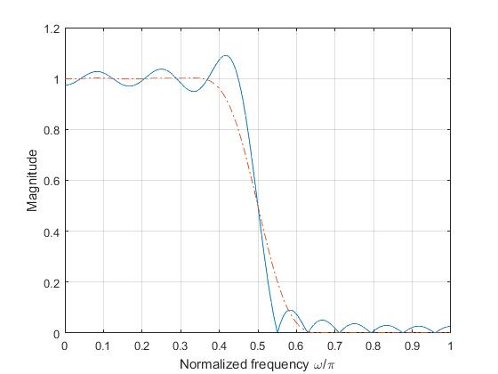
25-tap Lowpass Filter using Rectangular and Hamming Windows
The rectwin and hamming functions create the rectangular and Hamming window.

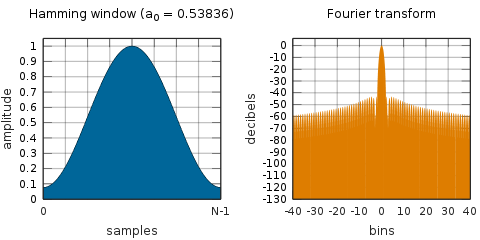
The Hamming window is generated from the equation: \[w(n) = 0.54 - 0.46 cos\left(2\pi\frac{n}{N}\right), \qquad 0 \le n \le N\] The window length \(L = N + 1\).
%% To design a 25-tap lowpass filter with cutoff frequency .5pi radians
% using rectangular and Hamming windows and plot their frequency response
wc = .5*pi;      % Cutoff frequency
N = 25; alpha = (N-1)/2; eps = .001;
n = 0:1:N-1;
hd = sin(wc*(n-alpha+eps))./(pi*(n-alpha+eps));
wr = rectwin(N); % Rectangular window sequence
hn = hd.*wr';    % Filter coefficients
w = 0:.01:pi;
h = freqz(hn,1,w);
plot(w/pi,abs(h)); hold on
wh = hamming(N); % Hamming window sequence
hn = hd.*wh';    % Filter coefficients
w = 0:.01:pi;
h = freqz(hn,1,w);
plot(w/pi,abs(h),'-.'); grid;
xlabel('Normalized frequency \omega/\pi');
ylabel('Magnitude'); hold off
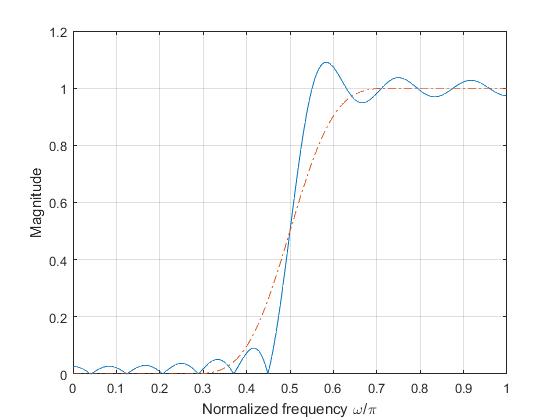
25-tap Highpass Filter using Rectangular and Blackman Windows
The blackman function creates the Blackman window.

The following equation defines the Blackman window of length \(N\): \[w(n) = 0.42 - 0.5 cos\frac{2\pi n}{N - 1} + 0.08cos\frac{4\pi n}{N - 1}, \] \[0 \le n \le M - 1\] where \(M\) is \(N/2\) for \(N\) even and \((N + 1)/2\) for \(N\) odd.
%% To design a 25-tap highpass filter with cutoff frequency .5pi radians
% using rectangular and Blackman windows and plot their frequency response
wc = .5*pi;      % Cutoff frequency
N = 25; alpha = (N-1)/2; eps = .001;
n = 0:1:N-1;
hd = (sin(pi*(n-alpha+eps)) - sin(wc*(n-alpha+eps))) ./ (pi*(n-alpha+eps));
wr = rectwin(N); % Rectangular window sequence
hn = hd.*wr';    % Filter coefficients
w = 0:.01:pi;
h = freqz(hn,1,w);
plot(w/pi,abs(h)); hold on
wh = blackman(N); % Blackman window sequence
hn = hd.*wh';     % Filter coefficients
w = 0:.01:pi;
h = freqz(hn,1,w);
plot(w/pi,abs(h),'-.'); grid;
xlabel('Normalized frequency \omega/\pi');
ylabel('Magnitude'); hold off
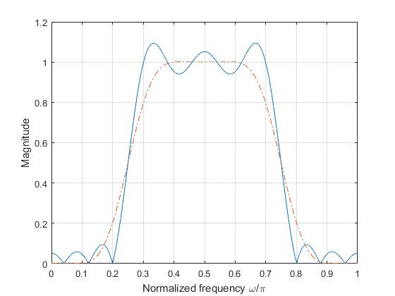
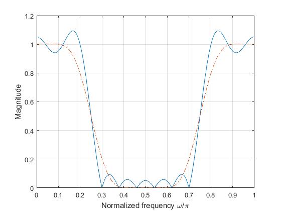
25-tap Bandpass Filter using Rectangular and Hamming Windows
%% To design a 25-tap bandpass filter with cutoff frequency .25pi and .75pi radians
% using rectangular and Hamming windows and plot their frequency response
wc1 = .25*pi; wc2 = .75*pi;      % Cutoff frequency
N = 25; a = (N-1)/2;
eps = .001; % To avoid indeterminate form
n = 0:1:N-1;
hd = (sin(wc2*(n-a+eps)) - sin(wc1*(n-a+eps))) ./ (pi*(n-a+eps));
wr = rectwin(N); % Rectangular window sequence
hn = hd.*wr';    % Filter coefficients
w = 0:.01:pi;
h = freqz(hn,1,w);
plot(w/pi,abs(h)); hold on
wh = hamming(N); % Hamming window sequence
hn = hd.*wh'; % Filter coefficients
w = 0:.01:pi;
h = freqz(hn,1,w);
plot(w/pi,abs(h),'-.'); grid;
xlabel('Normalized frequency \omega/\pi');
ylabel('Magnitude'); hold off
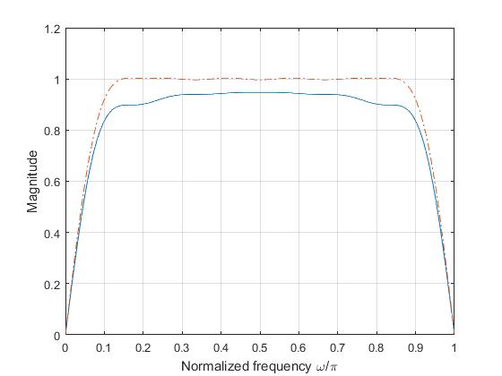
25-tap Bandstop Filter using Rectangular and Hamming Windows
%% To design a 25-tap bandstop filter with cutoff frequency .25pi and .75pi radians
% using rectangular and Hamming windows and plot their frequency response
wc1 = .25*pi; wc2 = .75*pi;      % Cutoff frequency
N = 25; a = (N-1)/2;
eps = .001; % To avoid indeterminate form
n = 0:1:N-1;
hd = (sin(wc1*(n-a+eps)) - sin(wc2*(n-a+eps)) + sin(pi*(n-a+eps))) ./ (pi*(n-a+eps));
wr = rectwin(N); % Rectangular window sequence
hn = hd.*wr';    % Filter coefficients
w = 0:.01:pi;
h = freqz(hn,1,w);
plot(w/pi,abs(h)); hold on
wh = hamming(N); % Hamming window sequence
hn = hd.*wh';    % Filter coefficients
w = 0:.01:pi;
h = freqz(hn,1,w);
plot(w/pi,abs(h),'-.'); grid;
xlabel('Normalized frequency \omega/\pi');
ylabel('Magnitude'); hold off
25-tap Hilbert Transformer using Bartlett and Hamming Windows

The coefficients of a Bartlett window are computed as follows: \[w(n) = \begin{cases} \frac{2n}{N}, & \text{\(0 \le n \le \frac{N}{2}\)} \\[2ex] 2-\frac{2n}{N}, & \text{\(\frac{N}{2} \le n \le N\)} \end{cases} \] The window length \(L = N + 1\).
%% To design a 25-tap Hilbert transformer using Bartlett
%  and Hamming windows and plot their frequency response
N = 25; a = (N-1)/2; eps = .001;
n = 0:1:N-1;
hd = (1 - cos(pi*(n-a+eps))) ./ (pi*(n-a+eps)); hd(a+1) = 0;
wt = bartlett(N); % Bartlett window
hn = hd.*wt';     % Filter coefficients
w = 0:.01:pi;
h = freqz(hn,1,w);
plot(w/pi,abs(h));   hold on
wh = hamming(N); % Hamming window sequence
hn = hd.*wh';    % Filter coefficients
w = 0:.01:pi;
h = freqz(hn,1,w);
plot(w/pi,abs(h),'-.'); grid;
xlabel('Normalized frequency \omega/\pi');
ylabel('Magnitude'); hold off
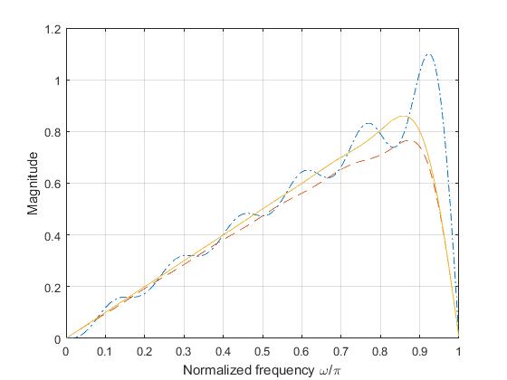
25-tap Differentiator using Rectangular, Bartlett and Hann Windows

The following equation generates the coefficients of a Hanning window: \[w(n) = 0.5\left(1−cos\left(2\pi\frac{n}{N}\right)\right), \qquad 0 \le n \le N\] The window length \(L = N + 1\).
%% To design a 25-tap differentiator using rectangular, Bartlett
%  and Hanning windows and plot their frequency response
N = 25; a = (N-1)/2; eps = .001;
n = 0:1:N-1;
hd = cos(pi*(n-a)) ./ (pi*(n-a)); hd(a+1) = 0;
wr = rectwin(N);  % rectangular window
hn = hd.*wr';     % Filter coefficients
w = 0:.01:pi;
h = freqz(hn,1,w);
plot(w/pi,abs(h),'-.'); hold on
wt = bartlett(N); % Bartlett window
hn = hd.*wt';     % Filter coefficients
w = 0:.01:pi;
h = freqz(hn,1,w);
plot(w/pi,abs(h),'--'); hold on
wh = hann(N); % Hanning window sequence
hn = hd.*wh'; % Filter coefficients
w = 0:.01:pi;
h = freqz(hn,1,w);
plot(w/pi,abs(h),'-');  grid;
xlabel('Normalized frequency \omega/\pi');
ylabel('Magnitude');    hold off
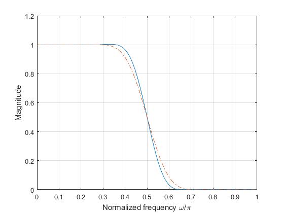
FIR Lowpass Filter using Hamming and Blackman Windows
The following equation defines the Blackman window of length N: \[w(n) = 0.42 − 0.5 cos\frac{2\pi n}{N - 1} + 0.08 cos\frac{4\pi n}{N - 1}, \] \[0 \le n \le M - 1\] where \(M\) is \(N/2 \) for \(N\) even and \((N + 1)/2 \) for \(N\) odd.
%% To design an FIR lowpass filter using Hamming and Blackman windows
wc = 0.5*pi; % Cutoff frequency
N = 25;
b = fir1(N,wc/pi,hamming(N+1));
w = 0:.01:pi;
h = freqz(b,1,w);
plot(w/pi,abs(h));   hold on
b = fir1(N,wc/pi,blackman(N+1));
w = 0:.01:pi;
h = freqz(b,1,w);
plot(w/pi,abs(h),'-.'); grid;
xlabel('Normalized frequency \omega/\pi');
ylabel('Magnitude'); hold off
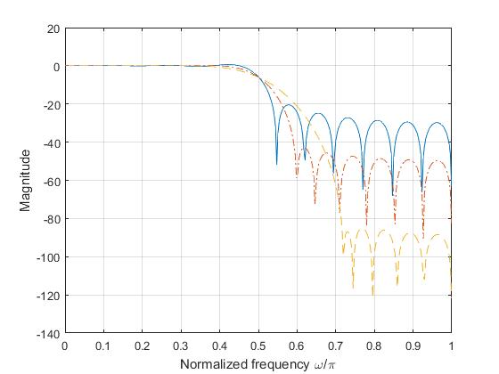
Lowpass Filter using Kaiser Window
 where \(\beta =^{def} \pi\alpha\).
The coefficients of a Kaiser window are computed from the following equation:
\[w(n) = \frac{I_0\left(\beta\sqrt{1 - \left(\frac{n - N/2}{N/2}\right)^2}\right)}{I_0(\beta)}, \qquad 0 \le n \le N\]
where \(I_0\) is the zeroth-order modified Bessel function of the first kind. The length \(L = N + 1\).
where \(\beta =^{def} \pi\alpha\).
The coefficients of a Kaiser window are computed from the following equation:
\[w(n) = \frac{I_0\left(\beta\sqrt{1 - \left(\frac{n - N/2}{N/2}\right)^2}\right)}{I_0(\beta)}, \qquad 0 \le n \le N\]
where \(I_0\) is the zeroth-order modified Bessel function of the first kind. The length \(L = N + 1\).
%% To plot the frequency response of lowpass filter using Kaiser window
%  for different values of beta
wc = 0.5*pi; % Cutoff frequency
N = 25;
b = fir1(N,wc/pi,kaiser(N+1,.5));   %Beta = .5
w = 0:.01:pi;
h = freqz(b,1,w);
plot(w/pi,20*log10(abs(h)));      hold on
b = fir1(N,wc/pi,kaiser(N+1,3.5));  %Beta = 3.5
w = 0:.01:pi;
h = freqz(b,1,w);
plot(w/pi,20*log10(abs(h)),'-.'); hold on
b = fir1(N,wc/pi,kaiser(N+1,8.5));  %Beta = 8.5
w = 0:.01:pi;
h = freqz(b,1,w);
plot(w/pi,20*log10(abs(h)),'--'); grid;
xlabel('Normalized frequency \omega/\pi');
ylabel('Magnitude');              hold off
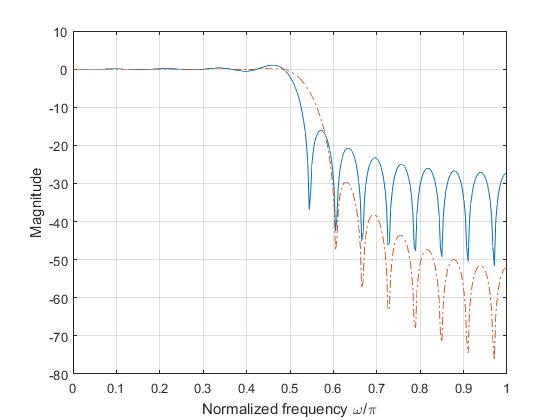
FIR Lowpass Filter using Frequency Sampling Method
%% To design a FIR lowpass filter with cutoff frequency .5pi using frequency sampling method
N = 33; % Number of samples
alpha = (N-1)/2;
Hrk = [ones(1,9), zeros(1,16), ones(1,8)]; % Samples of magnitude response
k1 = 0:(N-1)/2; k2 = (N+1)/2:N-1;
theta_k = [(-alpha*(2*pi)/N)*k1,(alpha*(2*pi)/N)*(N-k2)];
Hk = Hrk.*(exp(1i*theta_k));
hn = real(ifft(Hk,N));
w = 0:.01:pi;
H = freqz(hn,1,w);
plot(w/pi,20*log10(abs(H))); hold on
% FIR filter design using frequency sampling method with a transition sample
% at Hk(9) = 0.5 and Hk(24) = 0.5
Hrk = [ones(1,9), 0.5, zeros(1,14), 0.5, ones(1,8)]; % Samples of magnitude response
k1 = 0:(N-1)/2; k2 = (N+1)/2:N-1;
theta_k = [(-alpha*(2*pi)/N)*k1, (alpha*(2*pi)/N)*(N-k2)];
Hk = Hrk.*(exp(1i*theta_k));
hn = real(ifft(Hk,N));
w = 0:.01:pi;
H = freqz(hn,1,w);
plot(w/pi,20*log10(abs(H)),'-.'); grid;
xlabel('Normalized frequency \omega/\pi');
ylabel('Magnitude');         hold off
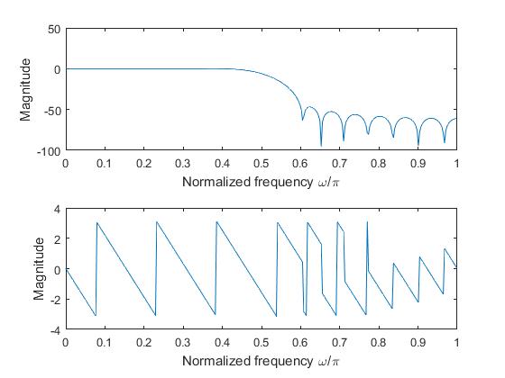
FIR Lowpass Filter using Kaiser Window
%% To design an FIR lowpass filter for the given specifications using Kaiser window
alphap = 0.1; % Passband attenuation in dB
alphas = 44;  % Stopband attenuation in dB
ws = 30;      % Stopband frequency in rad/sec
wp = 20;      % Passband frequency in rad/sec
wsf = 100;    % Sampling frequency in rad/sec
B = ws - wp;  % Transition width
wc = 0.5*(ws+wp);  % Cutoff frequency in rad/sec
wcr = wc*2*pi/wsf; % Cutoff drequenct=y in rad
D = (alphas - 7.95) / 14.36;
N = ceil((wsf*D/B)+1); % Order of the filter
alpha = (N-1) / 2
gamma = (.5842*(alphas-21).^(0.4)+0.07886*(alphas-21));
n = 0:1:N-1;
hd = sin(wcr*(n-alpha)) ./ (pi*(n-alpha)); hd(alpha+1) = 0.5;
wk = (kaiser(N,gamma))';
hn = hd.*wk;
w = 0:.01:pi;
h = freqz(hn,1,w);
subplot(2,1,1), plot(w/pi,20*log10(abs(h)))
xlabel('Normalized frequency \omega/\pi'); ylabel('Magnitude');
subplot(2,1,2), plot(w/pi,angle(h))
xlabel('Normalized frequency \omega/\pi'); ylabel('Magnitude');
This repo contains all the scripts used in this post. Here is a link to the previous part, a link to the first part and a link to the references part.