
Last semester, I had to take the course of Digital Signal Processing as a part of my ECE undergrad coursework. Unlike many other papers, to one’s awe, I didn’t find any reference site or portal, that would give me an overall review of the subject from an application-oriented viewpoint before being bogged down with its theories and practical assignments. Or that I could look up to, use as a reference site, to back up the learning process of this course throughout the semester.
The idea is to take an application-oriented practical approach towards the beautiful subject of DSP, that would help new learners taste its power, benefits before the theoretical knowledge takes over to complete it. Although, for gaining deep insights I do recommend thorough studying of textbooks, for which I would suggest the one authored by Professor John G. Proakis and Professor Dimitri G. Manokalis and the one by Sir Alan V. Oppenheim, which you can buy on Amazon from here and here.
Another purpose of this series of blog posts will be to function as an online reference for myself and other professionals in this field. I have tried to put together MATLAB algorithms of most of the topics covered in the standard DSP course at MIT OpenCourseWare. That being the reason, to keep the blog post from being extremely long and to keep you interested, I have split it into three segments along with a reference blog post, that indexes and describes shortly the set of functions I have used in this series and further readings and references.
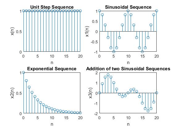
Generation of Discrete-Time Sequences
We use the mathematical functions for each of the known waveforms and subplot them in four sectors. In case of the unit step function, we create a row matrix of value ‘1’ using the ones function.
%% Generation of Discrete-Time Sequences
% Unit Step Sequence
N = 21;
x = ones(1,N);
n = 0:1:N-1;
subplot(2,2,1), stem(n,x);
xlabel('n'),ylabel('x(n)');
title('Unit Step Sequence');
%Sinusoidal Sequence
x1 = cos(.2*pi*n);
subplot(2,2,2), stem(n,x1);
xlabel('n'),ylabel('x1(n)');
title('Sinusoidal Sequence')
%Exponential Sequence
x2 = .8.^(n);
subplot(2,2,3), stem(n,x2);
xlabel('n'),ylabel('x2(n)');
title('Exponential Sequence')
%Addition of two Sinusoidal Sequence
x3 = sin(.1*pi*n) + sin(.2*pi*n);
subplot(2,2,4), stem(n,x3);
xlabel('n'),ylabel('x3(n)');
title('Addition of two Sinusoidal Sequences');
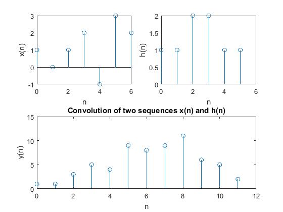
Convolution of Two Sequences
conv function does the job here.
%% Convolution of two sequences
x = [1,0,1,2,-1,3,2]; %Input Sequence
N1 = length(x);
n = 0:1:N1-1;
subplot(2,2,1), stem(n,x);
xlabel('n'), ylabel('x(n)');
h = [1,1,2,2,1,1]; %Impulse Sequence
N2 = length(h);
n1 = 0:1:N2-1;
subplot(2,2,2), stem(n1,h);
xlabel('n'), ylabel('h(n)');
y = conv(x,h) %Output Sequence
n2 = 0:1:N1+N2-2;
subplot(2,1,2), stem(n2,y);
xlabel('n'),ylabel('y(n)');
title('Convolution of two sequences x(n) and h(n)');
Command Window output:
y =
     1     1     3     5     4     9     8     9    11     6     5     2
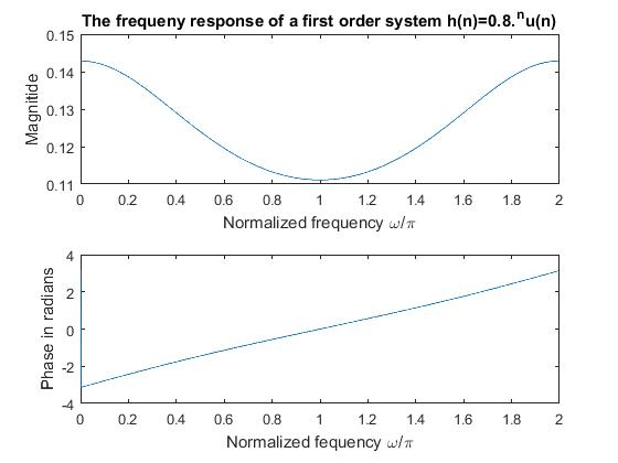
Frequency Response of a First Order System
The freqz function returns the frequency response vector \(h\), from the given values of the system \(H(z) = \frac{1}{1 - 8z^{-1}}\).
%% Frequency response of a first order system
b = [1]; %Numerator coefficients
a = [1,-8]; %Denominator coefficients
w = 0:0.01:2*pi;
[h] = freqz(b,a,w);
subplot(2,1,1), plot(w/pi,abs(h));
xlabel('Normalized frequency \omega/\pi'), ylabel('Magnitide');
title('The frequeny response of a first order system h(n)=0.8.^nu(n)');
subplot(2,1,2), plot(w/pi,angle(h));
xlabel('Normalized fequency \omega/\pi'), ylabel('Phase in radians');
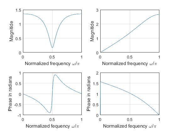
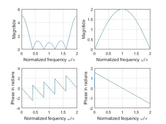
Frequency Response of Given Systems
The given systems are \(H(z) = \frac{1 + 0.9z^{-2}}{1 + 0.4z^{-2}}\) and \(H(z) = \frac{1 - z^{-1}}{1 + 0.25z^{-1}}\).
%% Frequency response of given systems
b = [1,0,.9]; %Numerator coefficients of system1
a = [1,0,.4]; %Denominator coefficients of system1
d = [1,-1]; %Numerator coefficients of system2
f = [1,.25]; %Denominator coefficients of system2
w = 0:.01:pi;
[h1] = freqz(b,a,w);
[h2] = freqz(d,f,w);
subplot(2,2,1), plot(w/pi,abs(h1));
xlabel('Normalized frequency \omega/\pi'), ylabel('Magnitide');grid
subplot(2,2,3), plot(w/pi,angle(h1));
xlabel('Normalized fequency \omega/\pi'), ylabel('Phase in radians');grid
subplot(2,2,2), plot(w/pi,abs(h2));
xlabel('Normalized frequency \omega/\pi'), ylabel('Magnitide');grid
subplot(2,2,4), plot(w/pi,angle(h2));
xlabel('Normalized fequency \omega/\pi'), ylabel('Phase in radians');grid
Frequency Response of FIR Systems
For the two FIR systems \(H(z) = 1 + z^{-1} + z^{-2} + z^{-3} + z^{-4}\) and \(H(z) = 1 - z^{-1}\).
%% Frequency response of FIR systems
b = ones(1,5); %FIR system1
a = [1];
d = [1,-1]; %FIR system2
f = [1];
w = 0:0.01:2*pi;
[h1] = freqz(b,a,w);
[h2] = freqz(d,f,w);
subplot(2,2,1), plot(w/pi,abs(h1));
xlabel('Normalized frequency \omega/\pi'), ylabel('Magnitide');grid
subplot(2,2,3), plot(w/pi,angle(h1));
xlabel('Normalized fequency \omega/\pi'), ylabel('Phase in radians');grid
subplot(2,2,2), plot(w/pi,abs(h2));
xlabel('Normalized frequency \omega/\pi'), ylabel('Magnitide');grid
subplot(2,2,4), plot(w/pi,angle(h2));
xlabel('Normalized fequency \omega/\pi'), ylabel('Phase in radians');grid
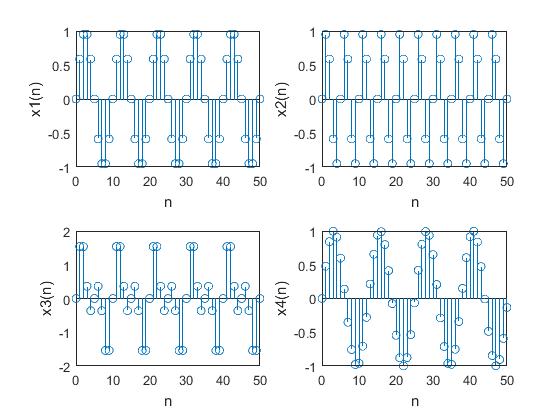
Periodic and Aperiodic Sequences
\(x4\) is the only aperiodic sequence here.
%% Periodic and aperiodic sequences
n = 0:1:50;
n1 = 0:1:50;
x1 = sin(.2*pi*n); %Sine wave with frequency w=0.2*pi
x2 = sin(.4*pi*n); %Sine wave with frequency w=0.4*pi
x3 = sin(.2*pi*n) + sin(.4*pi*n); %Sum of x1 and x2
x4 = sin(.5*n1); %Aperiodic sequence
subplot(2,2,1),stem(n,x1),xlabel('n'),ylabel('x1(n)'),axis([0 50 -1 1])
subplot(2,2,2),stem(n,x2),xlabel('n'),ylabel('x2(n)'),axis([0 50 -1 1])
subplot(2,2,3),stem(n,x3),xlabel('n'),ylabel('x3(n)'),axis([0 50 -2 2])
subplot(2,2,4),stem(n1,x4),xlabel('n'),ylabel('x4(n)'),axis([0 50 -1 1])
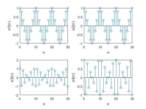
Periodicity Property of Digital Frequency
%% Periodicity property of digital frequency
n = 0:1:30;
x1 = cos(1.8*pi*n); %Sinewave with frequency w=1.8*pi
x2 = cos(.2*pi*n); %Sinewave with frequency w=0.2*pi
x3 = cos(1.1*pi*n); %Sinewave with frequency w=1.1*pi
x4 = cos(.9*pi*n); %Sinewave with frequency w=0.9*pi
subplot(2,2,1),stem(n,x1),xlabel('n'),ylabel('x1(n)'),axis([0 30 -1 1])
subplot(2,2,2),stem(n,x2),xlabel('n'),ylabel('x2(n)'),axis([0 30 -1 1])
subplot(2,2,3),stem(n,x3),xlabel('n'),ylabel('x3(n)'),axis([0 30 -2 2])
subplot(2,2,4),stem(n,x4),xlabel('n'),ylabel('x4(n)'),axis([0 30 -1 1])
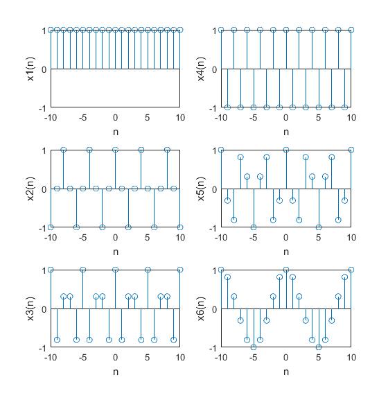
Demonstration of the Property of Digital Frequency
%% Property of digital frequency
n = -10:1:10;
x1 = cos(0*pi*n); %Sinewave with frequency w=0
x2 = cos(.5*pi*n); %Sinewave with frequency w=0.5*pi
x3 = cos(.8*pi*n); %Sinewave with frequency w=0.8*pi
x4 = cos(pi*n); %Sinewave with frequency w=pi
x5 = cos(1.4*pi*n); %Sinewave with frequency w=1.4*pi
x6 = cos(1.8*pi*n); %Sinewave with frequency w=1.8*pi
subplot(3,2,1),stem(n,x1),xlabel('n'),ylabel('x1(n)'),axis([-10 10 -1 1])
subplot(3,2,3),stem(n,x2),xlabel('n'),ylabel('x2(n)'),axis([-10 10 -1 1])
subplot(3,2,5),stem(n,x3),xlabel('n'),ylabel('x3(n)'),axis([-10 10 -1 1])
subplot(3,2,2),stem(n,x4),xlabel('n'),ylabel('x4(n)'),axis([-10 10 -1 1])
subplot(3,2,4),stem(n,x5),xlabel('n'),ylabel('x5(n)'),axis([-10 10 -1 1])
subplot(3,2,6),stem(n,x6),xlabel('n'),ylabel('x6(n)'),axis([-10 10 -1 1])
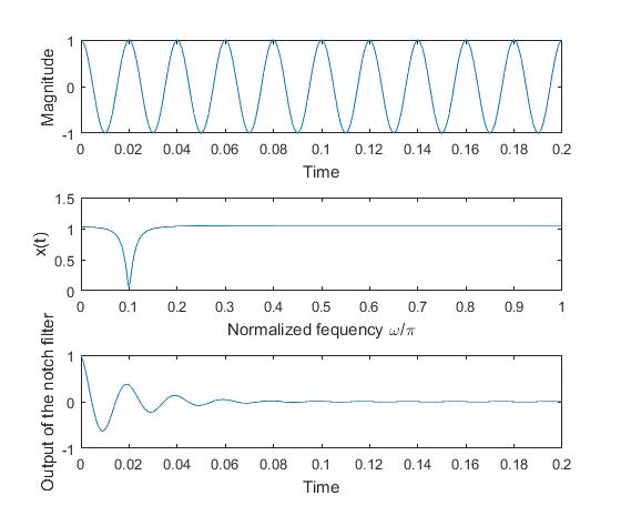
A Notch Filter that filters 50 Hz Noise
The filter works on the basis of the given values of coefficients of the numerator and the denominator of the transfer function.
%% 50Hz noise filter
t = 0:.001:2;
x = cos(2*pi*50*t);
x1 = cos(2*pi*50*t);
b = [1 -1.9022 1]; a = [1 -1.8072 .9025]; %Filter coefficients
y = filter(b,a,x);
w = 0:.01:pi;
h = freqz(b,a,w);
subplot(3,1,2),plot(w/pi,abs(h)),xlabel('Normalized fequency \omega/\pi'),ylabel('x(t)'),axis([0 1 0 1.5])
subplot(3,1,1),plot(t,x),xlabel('Time'),ylabel('Magnitude'),axis([0 .2 -1 1])
subplot(3,1,3),plot(t,y),xlabel('Time'),ylabel('Output of the notch filter'),axis([0 .2 -1 1])
This repo contains all the scripts used in this post. Here is a link to the next part.