
A link to the previous part, a link to the next part and a link to the references part.
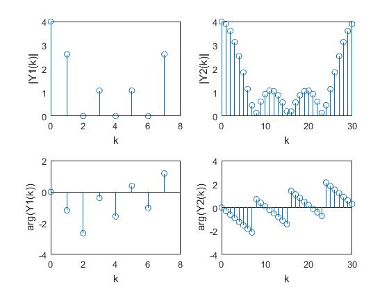
DFT of a Sequence - Magnitude and Phase Response
The function takes the input sequence and the number of frequency points as two arguments.
%% DFT of a sequence and plot of the magnitude and phase response
x = ones(1,4); %Input sequence
N1 = 8; %Number of frequency points
Y1 = dft(x,N1)
k = 0:1:N1-1;
subplot(2,2,1), stem(k,abs(Y1)), xlabel('k'), ylabel('|Y1(k)|');
subplot(2,2,3), stem(k,angle(Y1)), xlabel('k'), ylabel('arg(Y1(k))');
N2 = 31 %Number of frequency points
Y2 = dft(x,N2)
k = 0:1:N2-1;
subplot(2,2,2), stem(k,abs(Y2)), xlabel('k'), ylabel('|Y2(k)|');
subplot(2,2,4), stem(k,angle(Y2)), xlabel('k'), ylabel('arg(Y2(k))');
dft.m:
function X = dft(xn,N)
% To compute the DFT of the sequence x(n)
L = length(xn); %Length of the sequence
%Checking for the length of the DFT
if(N<L)
    error('N must be >=L')
end
x1 = [xn zeros(1,N-L)]; %Appending zeros
%Computation of twiddle factors
for k = 0:1:N-1
    for n = 0:1:N-1
        p = exp(-i*2*pi*n*k/N);
        x2(k+1,n+1) = p;
    end
end
X = x1 * x2;
Notice that the Command Window shows the two output sequences of the 8-point and 50-point DFT.
Inverse DFT of a Sequence
%% Inverse DFT of a sequence
X = [4,1+i,0,1,-i,0,1+i,1-i];
N = length(X);
xn = idft(X,N)
idft.m:
function xn = idft(X,N)
%To compute the inverse DFT of the sequence X(k)
L = length(X); %Length of the sequence
%Computation of twiddle factors
for k = 0:1:N-1
    for n = 0:1:N-1
        p = exp(i*2*pi*n*k/N);
        x2(k+1,n+1) = p;
    end
end
xn = (X*x2.')/N;
Command Window output:
xn =
  Columns 1 through 7
   1.0000 + 0.0000i   0.5366 + 0.0884i   0.1250 - 0.3750i   0.1098 + 0.3384i   0.2500 + 0.0000i   0.7134 - 0.0884i   0.6250 - 0.1250i
  Column 8
   0.6402 + 0.1616i
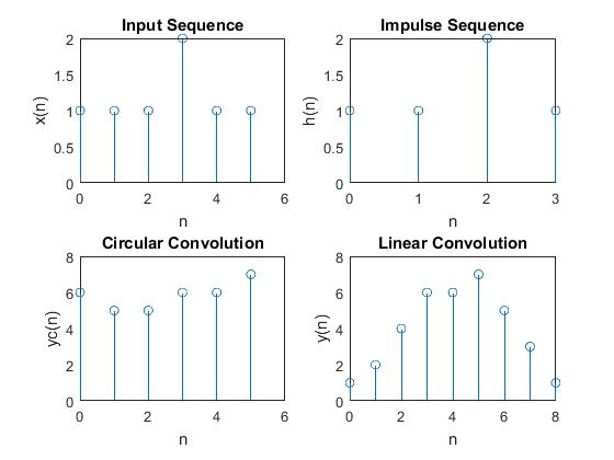
Circular Convolution of two Sequences
%% Circular convolution of two sequences
n = 0:7;
x = sin(3*pi*n/8); % Input sequence 1
h = [1,1,1,1]; % Input sequence 2
Nx = length(x);
Nh = length(h);
N = 8;
if(N<max(Nx,Nh))
    error('N must be >=max(Nx,Nh')
end
y = circconv(x,h,N)
circconv.m:
function [y] = circconv(x,h,N);
% To find the circular convolution of two sequences
% x = input sequence 1
% h = impulse sequence 2
% N = Number of points in the output sequence
N2 = length(x);
N3 = length(h);
x = [x zeros(1,N-N2)] %Append N-N2 zeros to the input sequence 1
h = [h zeros(1,N-N3)] %Append N-N3 zeros to the sequence 2
% circular shift of the sequence 2
m = [0:1:N-1];
M = mod(-m,N);
h = h(M+1);
for n = 1:1:N
    m = n-1;
    p = 0:1:N-1;
    q = mod(p-m,N);
    hm = h(q+1);
    H(n,:) = hm;
end
% Matrix convolution
y = x*H';
Command Window output:
x =
         0    0.9239    0.7071   -0.3827   -1.0000   -0.3827    0.7071    0.9239
h =
     1     1     1     1     0     0     0     0
y =
    1.2483    2.5549    2.5549    1.2483    0.2483   -1.0583   -1.0583    0.2483
Comparison between Circular and Linear Convolutions of two Sequences
%% Frequency response of given systems
b = [1,0,.9]; %Numerator coefficients of system1
a = [1,0,.4]; %Denominator coefficients of system1
d = [1,-1]; %Numerator coefficients of system2
f = [1,.25]; %Denominator coefficients of system2
w = 0:.01:pi;
[h1] = freqz(b,a,w);
[h2] = freqz(d,f,w);
subplot(2,2,1), plot(w/pi,abs(h1));
xlabel('Normalized frequency \omega/\pi'), ylabel('Magnitide');grid
subplot(2,2,3), plot(w/pi,angle(h1));
xlabel('Normalized fequency \omega/\pi'), ylabel('Phase in radians');grid
subplot(2,2,2), plot(w/pi,abs(h2));
xlabel('Normalized frequency \omega/\pi'), ylabel('Magnitide');grid
subplot(2,2,4), plot(w/pi,angle(h2));
xlabel('Normalized fequency \omega/\pi'), ylabel('Phase in radians');grid
Overlap and Save Method
%% Overlap and save method
x = [1,2,-1,2,3,-2,-3,-1,1,1,2,-1]; % Input sequence
h = [1,2,1,1]; % Impulse sequence
N = 4; % Length of each block before appending zeros
y = ovrlsav(x,h,N);
ovrlsav.m:
function y = ovrlsav(x,h,N)
% To compute the output of a system using overlap and save method
% x = input seuence
% h = impulse sequence
% N = Length of each block
if(N<length(h))
    error('N must be >=length(h)')
end
Nx = length(x);
M = length(h);
M1 = M-1;
L = N-M1;
x = [zeros(1,M-1),x,zeros(1,N-1)];
h = [h zeros(1,N-M)];
K = floor((Nx+M1-1)/(L)); % Number of blocks
Y = zeros(K+1,N);
%Dividing the sequence into two blocks
for k = 0:K
    xk = x(k*L+1:k*L+N);
    Y(k+1,:) = circconv(xk,h,N);
end
Y = Y(:,M:N)'; %Discard first M-1 blocks
y = (Y(:))'
Command Window output:
y =
     1     4     4     3     8     5    -2    -6    -6    -1     4     5     1     1    -1
Overlap and Add Method
%% Overlap and add method
x = [1,2,-1,2,3,-2,-3,-1,1,1,2,-1]; %Input sequence
h = [1,2,1,1]; %Impulse sequence
L = 4; %Length of each block before appending zeros
y = ovrladd(x,h,L);
ovrladd.m:
function y = ovrladd(x,h,L)
% To compute the output of a system using overlap and add method
% x = input sequence
% h = impulse sequence
% L = Length of each block
Nx = length(x);
M = length(h);
M1 = M-1;
R = rem(Nx,L);
N = L+M1;
x = [x zeros(1,L-R)];
h = [h zeros(1,N-M)];
K = floor(Nx/L); % Number of blocks
Y = zeros(K+1,N);
z = zeros(1,M1);
% Dividing the sequence into K blocks
for k = 0:K
    xp = x(k*L+1:k*L+L);
    xk = [xp z];
    y(k+1,:) = circconv(xk,h,N);
end
yp = y';
[x,y] = size(yp);
for i = L+1:x
    for j=1:y-1
        temp1 = i-L;
        temp2 = j+1;
        temp3 = yp(temp1,temp2)+yp(i,j);
        yp(temp1,temp2) = yp(i,j);
        yp(temp1,temp2) = temp3;
    end
end
z = 1;
for j = 1:y
    for i = 1:x
        if((i<=L && j<=y-1)||(j==y))
            ypnew(z) = yp(i,j);
            z = z+1;
        end
    end
end
y = ypnew
Command Window output:
y =
     1     4     4     3     8     5    -2    -6    -6    -1     4     5     1     1    -1     0     0     0     0
Butterworth Lowpass Filter
The buttord and butter functions can be used while designing a Butterworth filter.
%% To design a Butterworth lowpass filter for the specifications
alphap = .4;  %Passband attenuation in dB
alphas = 30;  %Stopband attenuation in dB
fp = 400;     %Passband frequency in Hz
fs = 800;     %Stopband frequency in Hz
F = 2000;     %Sampling frequency in Hz
omp = 2*fp/F;
oms = 2*fs/F;
%To find cutoff frequency and order of the filter
[n,wn] = buttord(omp,oms,alphap,alphas);
%system function of the filter
[b,a] = butter(n,wn)
w = 0:.01:pi;
[h,om] = freqz(b,a,w,'whole');
m = abs(h);
an = angle(h);
subplot(2,1,1); plot(om/pi,20*log(m)); grid; xlabel('Normalized frequency'); ylabel('Gain in dB');
subplot(2,1,2); plot(om/pi,an);        grid; xlabel('Normalized frequency'); ylabel('Phase in radians');
Command Window output:
b =
    0.1518    0.6073    0.9109    0.6073    0.1518
a =
    1.0000    0.6418    0.6165    0.1449    0.0259

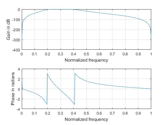
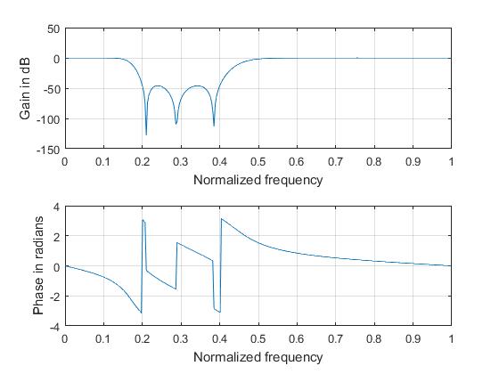
Butterworth Bandpass Filter
%% To design a Butterworth bandpass filter for the specifications
alphap = 2;         %Pass band attenuation in dB
alphas = 20;        %Stop band attenuation in dB
wp = [.2*pi,.4*pi]; %Passband frequency in radians
ws = [.1*pi,.5*pi]; %Stopband frequency in radians
%To find cutoff frequency and order of the filter
[n,wn] = buttord(wp/pi,ws/pi,alphap,alphas);
%System function of the filter
[b,a] = butter(n,wn)
w = 0:.01:pi;
[h,ph] = freqz(b,a,w);
m = 20*log10(abs(h));
an = angle(h);
subplot(2,1,1); plot(ph/pi,m); grid; xlabel('Normalized frequency'); ylabel('Gain in dB');
subplot(2,1,2); plot(ph/pi,an); grid; xlabel('Normalized frequency'); ylabel('Phase in radians');
Command Window output:
b =
    0.0060         0   -0.0240         0    0.0359         0   -0.0240         0    0.0060
a =
    1.0000   -3.8710    7.9699  -10.6417   10.0781   -6.8167    3.2579   -1.0044    0.1670
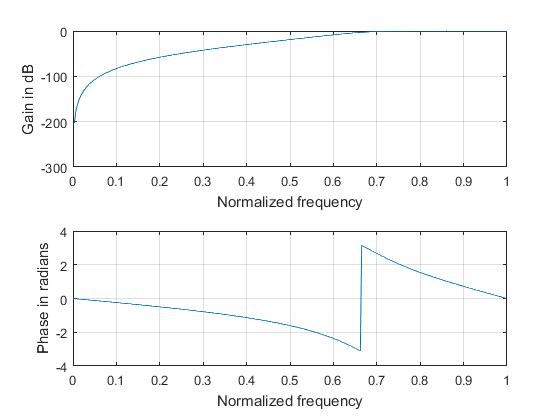
Butterworth Highpass Filter
%% To design a Butterworth highpass filter for the specifications
alphap = .4;        % Pass band attenuation in dB
alphas = 30;        % Stop band attenuation in dB
fp = 800;           % Passband frequency in radians
fs = 400;           % Stopband frequency in radians
F = 2000;           % Sampling frequency in Hz
omp = 2*fp/F;
oms = 2*fs/F;
%To find cutoff frequency and order of the filter
[n,wn] = buttord(omp,oms,alphap,alphas);
%system function of the filter
[b,a] = butter(n,wn,'high')
w = 0:.01:pi;
[h,om] = freqz(b,a,w);
m = 20*log10(abs(h));
an = angle(h);
subplot(2,1,1); plot(om/pi,m);  grid; xlabel('Normalized frequency'); ylabel('Gain in dB');
subplot(2,1,2); plot(om/pi,an); grid; xlabel('Normalized frequency'); ylabel('Phase in radians');
Command Window output:
b =
    0.0265   -0.1058    0.1587   -0.1058    0.0265
a =
    1.0000    1.2948    1.0206    0.3575    0.0550
Butterworth Band-stop Filter
%% To design a Butterworth bandstop filter for the specifications
alphap = 2;         % Pass band attenuation in dB
alphas = 20;        % Stop band attenuation in dB
ws = [.2*pi,.4*pi]; % Stopband frequency in radians
wp = [.1*pi,.5*pi]; % Passband frequency in radians
%To find cutoff frequency and order of the filter
[n,wn] = buttord(wp/pi,ws/pi,alphap,alphas);
%System function of the filter
[b,a] = butter(n,wn,'stop')
w = 0:.01:pi;
[h,ph] = freqz(b,a,w);
m = 20*log10(abs(h));
an = angle(h);
subplot(2,1,1); plot(ph/pi,m);  grid; xlabel('Normalized frequency'); ylabel('Gain in dB');
subplot(2,1,2); plot(ph/pi,an); grid; xlabel('Normalized frequency'); ylabel('Phase in radians');
Command Window output:
b =
    0.2348   -1.1611    3.0921   -5.2573    6.2629   -5.2573    3.0921   -1.1611    0.2348
a =
    1.0000   -3.2803    5.4917   -6.1419    5.0690   -3.0524    1.3002   -0.3622    0.0558
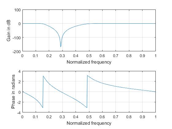
Chebyshev Type I Lowpass Filter
Likewise, the cheb1ord and cheby1 functions can be used while designing a Chebyshev type I filter.
%% To design a Chebyshev 1 lowpass filter for the specifications
alphap = 1;  %Pass band attenuation in dB
alphas = 15; %Stop band attenuation in dB
wp = .2*pi;  %Pass band frequency in radians
ws = .3*pi;  %Stop band frequency in radians
%To find cutoff frequency and order of the filter
[n,wn] = cheb1ord(wp/pi,ws/pi,alphap,alphas);
%System function of the filter
[b,a] = cheby1(n,alphap,wn)
w = 0:.01:pi;
[h,ph] = freqz(b,a,w);
m = 20*log(abs(h));
an = angle(h);
subplot(2,1,1); plot(ph/pi,m);  grid; xlabel('Normalized frequency'); ylabel('Gain in dB');
subplot(2,1,2); plot(ph/pi,an); grid; xlabel('Normalized frequency'); ylabel('Phase in radians');
Command Window output:
b =
    0.0018    0.0073    0.0110    0.0073    0.0018
a =
    1.0000   -3.0543    3.8290   -2.2925    0.5507
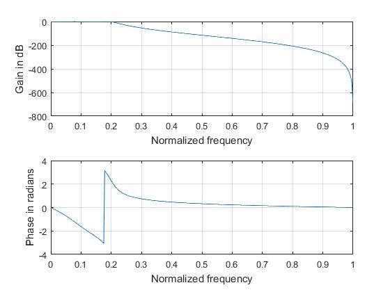
Chebyshev Type II Lowpass Filter
Here cheb2ord and cheby2 are used.
%% To design a Chebyshev 2 lowpass filter for the specifications
alphap = 1;  %Pass band attenuation in dB
alphas = 20; %Stop band attenuation in dB
wp = .2*pi;  %Pass band frequency in radians
ws = .3*pi;  %Stop band frequency in radians
%To find cutoff frequency and order of the filter
[n,wn] = cheb2ord(wp/pi,ws/pi,alphap,alphas);
%System function of the filter
[b,a] = cheby2(n,alphas,wn)
w = 0:.01:pi;
[h,ph] = freqz(b,a,w);
m = abs(h);
an = angle(h);
subplot(2,1,1); plot(ph/pi,20*log(m)); grid; xlabel('Normalized frequency'); ylabel('Gain in dB');
subplot(2,1,2); plot(ph/pi,an);        grid; xlabel('Normalized frequency'); ylabel('Phase in radians');
Command Window output:
b =
    0.1160   -0.0591    0.1630   -0.0591    0.1160
a =
    1.0000   -1.8076    1.5891   -0.6201    0.1153
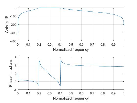
Chebyshev Type I Bandpass Filter
%% To design a Chebyshev 1 bandpass filter for the specifications
alphap = 2;  %Pass band attenuation in dB
alphas = 20; %Stop band attenuation in dB
wp = [.2*pi,.4*pi];  %Pass band frequency in radians
ws = [.1*pi,.5*pi];  %Stop band frequency in radians
%To find cutoff frequency and order of the filter
[n,wn] = cheb1ord(wp/pi,ws/pi,alphap,alphas);
%System function of the filter
[b,a] = cheby1(n,alphap,wn)
w = 0:.01:pi;
[h,ph] = freqz(b,a,w);
m = 20*log10(abs(h));
an = angle(h);
subplot(2,1,1); plot(ph/pi,m);  grid; xlabel('Normalized frequency'); ylabel('Gain in dB');
subplot(2,1,2); plot(ph/pi,an); grid; xlabel('Normalized frequency'); ylabel('Phase in radians');
Command Window output:
b =
    0.0083         0   -0.0248         0    0.0248         0   -0.0083
a =
    1.0000   -3.2632    5.9226   -6.6513    5.0802   -2.3909    0.6307
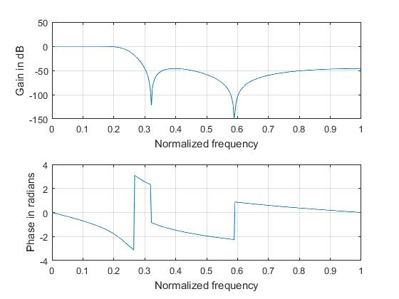
Chebyshev Type II Bandstop Filter
%% To design a Chebyshev 2 bandstop filter for the specifications
alphap = 2;  %Pass band attenuation in dB
alphas = 20; %Stop band attenuation in dB
ws = [.2*pi,.4*pi];  %Stop band frequency in radians
wp = [.1*pi,.5*pi];  %Pass band frequency in radians
%To find cutoff frequency and order of the filter
[n,wn] = cheb2ord(wp/pi,ws/pi,alphap,alphas);
%System function of the filter
[b,a] = cheby2(n,alphas,wn,'stop')
w = 0:.01:pi;
[h,ph] = freqz(b,a,w);
m = 20*log(abs(h));
an = angle(h);
subplot(2,1,1); plot(ph/pi,m);  grid; xlabel('Normalized frequency'); ylabel('Gain in dB');
subplot(2,1,2); plot(ph/pi,an); grid; xlabel('Normalized frequency'); ylabel('Phase in radians');
Command Window output:
b =
    0.4870   -1.7177    3.3867   -4.1110    3.3867   -1.7177    0.4870
a =
    1.0000   -2.7289    4.0090   -3.7876    2.5028   -1.0299    0.2357
Conversion of an Analog Filter into a Digital Filter using Impulse Invariance Method
This is a direct implementation of the impinvar function.
%% To convert the analog filter into digital filter using impulse invariance
b = [1,2];       % Numerator coefficients of analog filter
a = [1,5,11,15]; % Denominator coefficients of analog filter
f = 5;           % Sampling frequency
[bz,az] = impinvar(b,a,f)
Command Window output:
bz =
    0.0000    0.0290   -0.0195
az =
    1.0000   -2.0570    1.4980   -0.3679
Conversion of an Analog Filter into a Digital Filter using Bilinear Transformation
bilinear here.
%% To convert the analog filter into digital filter using bilinear transformation
b = [2];     % Numerator coefficients of analog filter
a = [1,3,2]; % Denominator coefficients of analog filter
f = 1;       % Sampling frequency
[bz,az] = bilinear(b,a,f)
Command Window output:
bz =
    0.1667    0.3333    0.1667
az =
    1.0000   -0.3333    0.0000
This repo contains all the scripts used in this post. Here is a link to the previous part, a link to the next part and a link to the references part.